Run pavo's adjacency and boundary strength analysis on a recolorize object
Source: R/recolorize_adjacency.R
recolorize_adjacency.RdRun adjacency (Endler 2012) and boundary strength (Endler et al. 2018)
analysis directly on a recolorize object, assuming a human viewer
(i.e. using CIE Lab and HSL color distances that correspond to
perceptual distances of human vision). This is achieved by
converting the recolorize object to a pavo::classify object,
converting the colors to HSL space, and calculating a pavo::coldist object
for CIE Lab color space before running pavo::adjacent.
Arguments
- recolorize_obj
A
recolorizeobject.- xscale
The length of the x-axis, in preferred units. Passed to pavo::adjacent.
- coldist
A pavo::coldist object; otherwise, this argument is ignored and a
coldistobject for human vision is calculated from RGB colors converted to CIE Lab using cielab_coldist.- hsl
A dataframe with
patch,hue,satandlumcolumns specifying the HSL values for each color patch, to be passed to pavo::adjacent. Otherwise, this argument is ignored and HSL values are calculated for human vision from the RGB colors in therecolorizeobject.- ...
Further arguments passed to pavo::adjacent.
Value
The results of pavo::adjacent; see that documentation for the meaning of each specific value.
Details
Eventually, the plan is to incorporate more sophisticated color models than using human perceptual color distances, i.e. by allowing users to match color patches to spectra. However, this does return reasonable and informative results so long as human vision is an appropriate assumption for the image data.
Examples
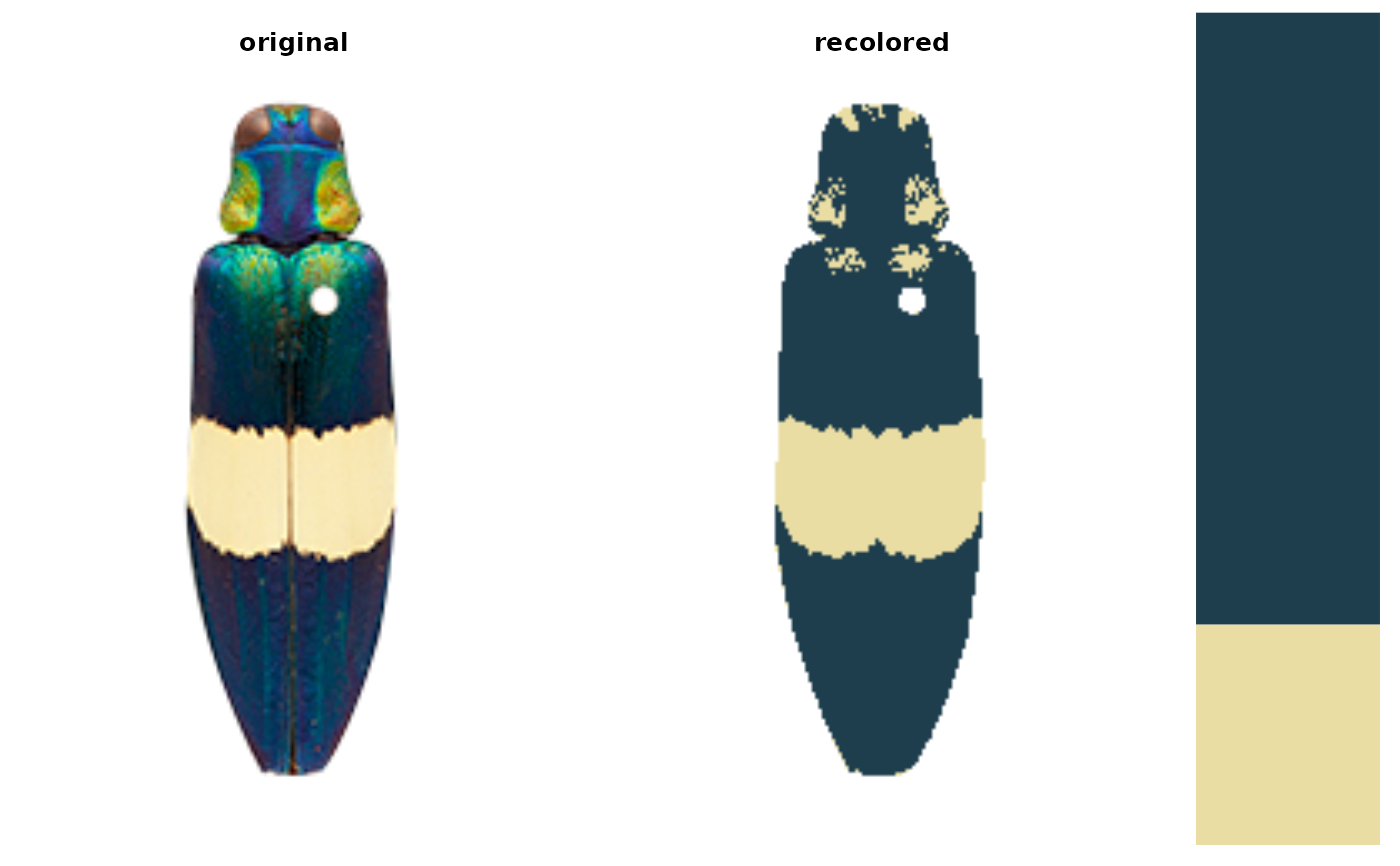
img <- system.file("extdata/chongi.png", package = "recolorize")
recolorize_obj <- recolorize(img, method = "k", n = 2)

recolorize_adjacency(recolorize_obj)
#> Using single set of coldists for all images.
#> Using single set of hsl values for all images.
#>  k     N n_off       p_1       p_2       p_3     q_1_1       q_1_2     q_2_2
#>  3 40364  1340 0.5150934 0.1287119 0.3561947 0.5041869 0.003121593 0.1186701
#>     q_1_3      q_2_3     q_3_3      t_1_2     t_1_3     t_2_3        m     m_r
#>  0.011099 0.01897731 0.3439451 0.09402985 0.3343284 0.5716418 2.964602 3.50885
#>       m_c        A       Sc       St        Jc        Jt         B        Rt
#>  2.420354 1.449726 2.446408 2.235179 0.8154692 0.7450598 0.3134328 0.4473914
#>  Rab     m_dS     s_dS    cv_dS     m_dL     s_dL     cv_dL     m_hue    s_hue
#>    1 31.90773 17.47305 0.547612 62.60339 23.13469 0.3695437 0.5307585 1.605562
#>    var_hue     m_sat     s_sat   cv_sat     m_lum     s_lum    cv_lum
#>  0.7244305 0.2508135 0.3565633 1.421627 0.6910565 0.4721701 0.6832583